
Introduction
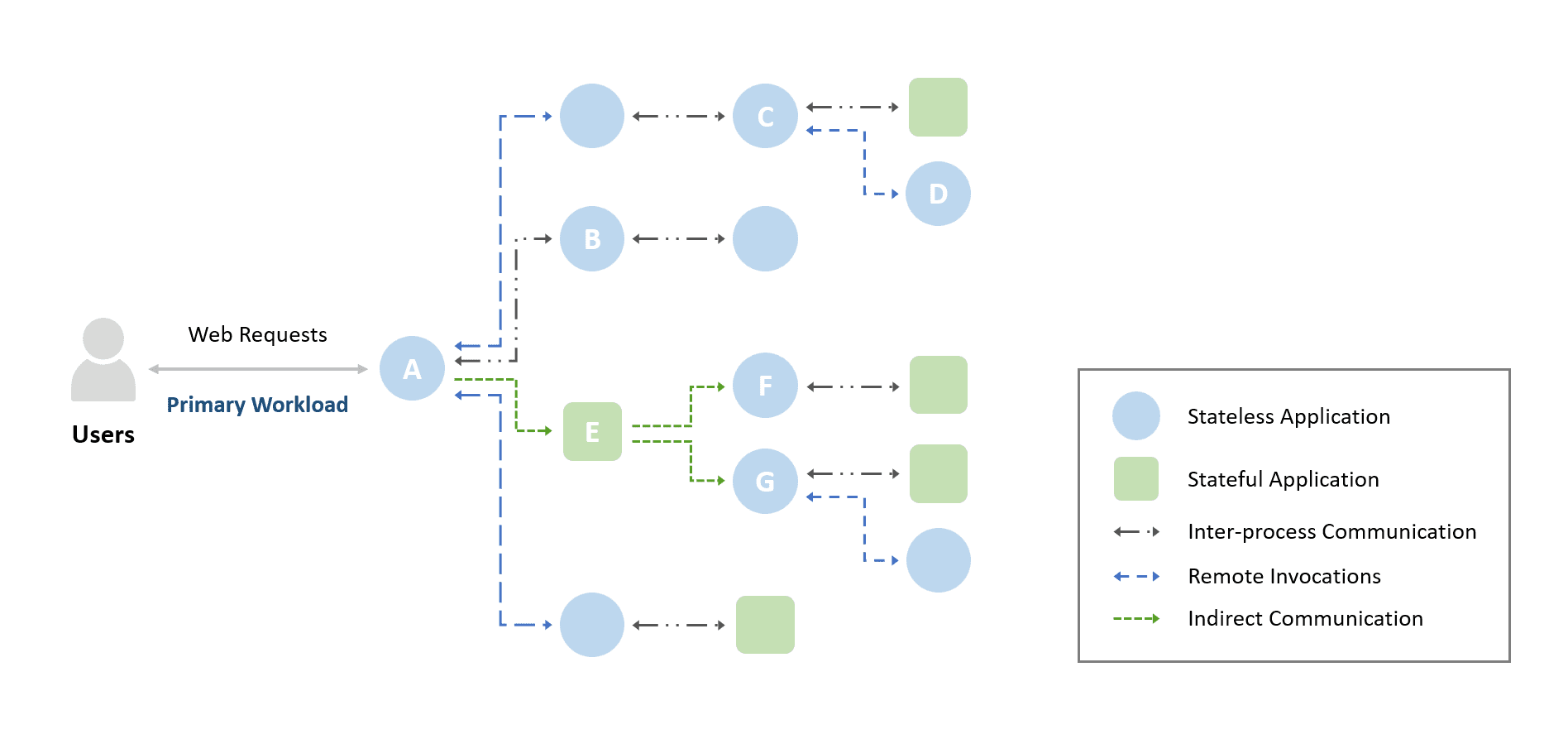
Deploying applications in a serverless cloud platform or a Kubernetes system in the cloud has become a popular option for users. Figure 1 is an illustration of an example of a microservice architecture. Usually, web requests sent to a web server are forwarded to the various microservices behind, and they trigger a series of communications between related microservices. Since the number of web requests to the webserver represents the workload of this entire application, we name it the Primary Workload. As shown in Figure 1, these microservices include stateless microservices such as web servers and stateful microservices such as databases. There are complicated and complex communications between these microservices, for example, inter-process communications, remote invocations, or indirect communications [1]. A webserver (MS-A) sends data to the backend database (MS-B), an example of inter-process communications. An example of remote invocations is the two-way communications between the downstream microservice (MS-C) and its upstream microservice (MS-D), and an example of indirect communications is the traffic from message consumers (MS-F and MS-G) consuming messages from a message queue (MS-E). These communication behaviors between applications in a microservice system introduce a variety of workload patterns, especially for a serverless cloud platform [2].
Prediction-based Resource Management
For typical resource management of an application with many microservices deployed in a Kubernetes system, it is desired to allocate the right amount of resources to all the microservices so that performance would not be suffered because of resource constraints and, at the same time, no wasted expenses for excessive allocations. There are several benefits of utilizing predictions when considering resource management for microservice-based applications. First, predictions based on the past workload patterns provide a better forecast for resource usage patterns of microservices. It gives an insight into how many resources will be used at what time by a microservice. Second, the workload prediction will be very beneficial when considering autoscaling some stateless microservices. For example, the system can continuously predict the workload of a stateless microservice every few minutes and proactively scale this microservice in time for the upcoming workload.
There are some factors to consider when adopting prediction-based resource management for applications deployed in a Kubernetes environment. For example, generating 100 workload predictions every minute requires an average runtime per the prediction of about 0.6s with a minor resource impact on computation costs introduced by predictions. In addition, microservices in Kubernetes may be restarted, failed, or terminated for some reason. This would cause unusual patterns like change points or unpredictable events. Therefore, using predictions for resource management in a Kubernetes system needs to handle these unusual patterns for a good result.
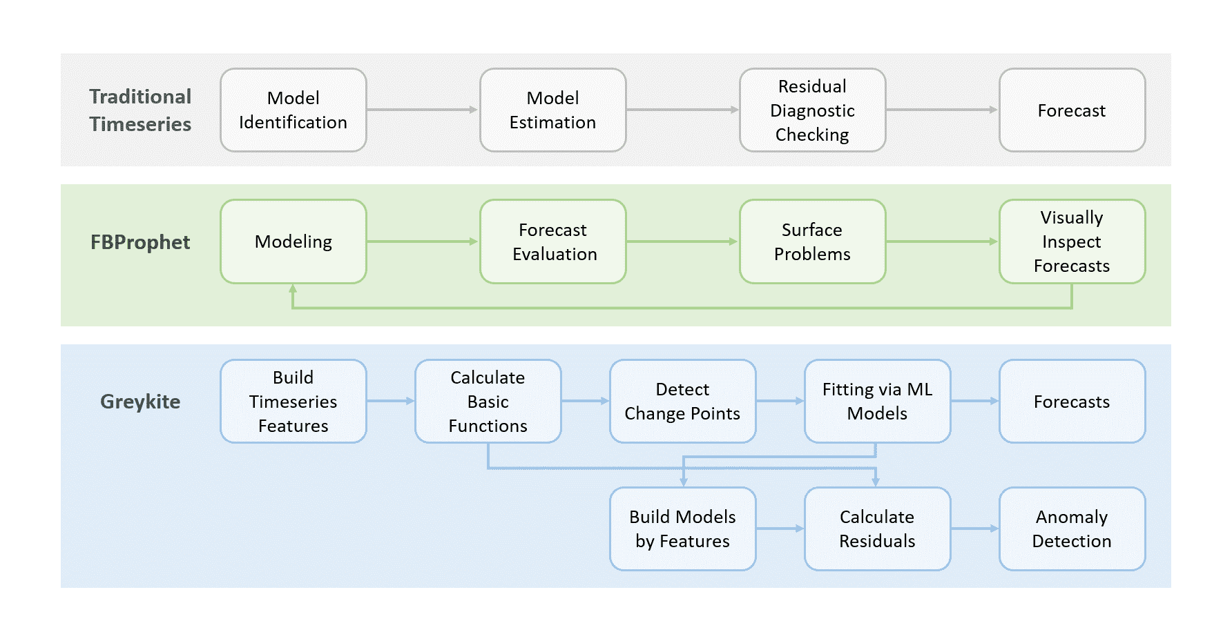
Figure 2 shows the prediction steps of traditional time series schemes. There are four steps in modeling time series data: model identification, model estimation, residual diagnostic checking, and forecasting [3]. When users want to generate a forecast for a microservice workload, they need to preprocess missing values and identify the specific model orders for the workload metric in advance. Next, users would estimate these model parameters, find a suitable model for predictions, and check whether the model is overfitting or not by the residual diagnostic checking step. Finally, users start to generate predictions for the microservice workload.
Predictions Based on Cross-correlations
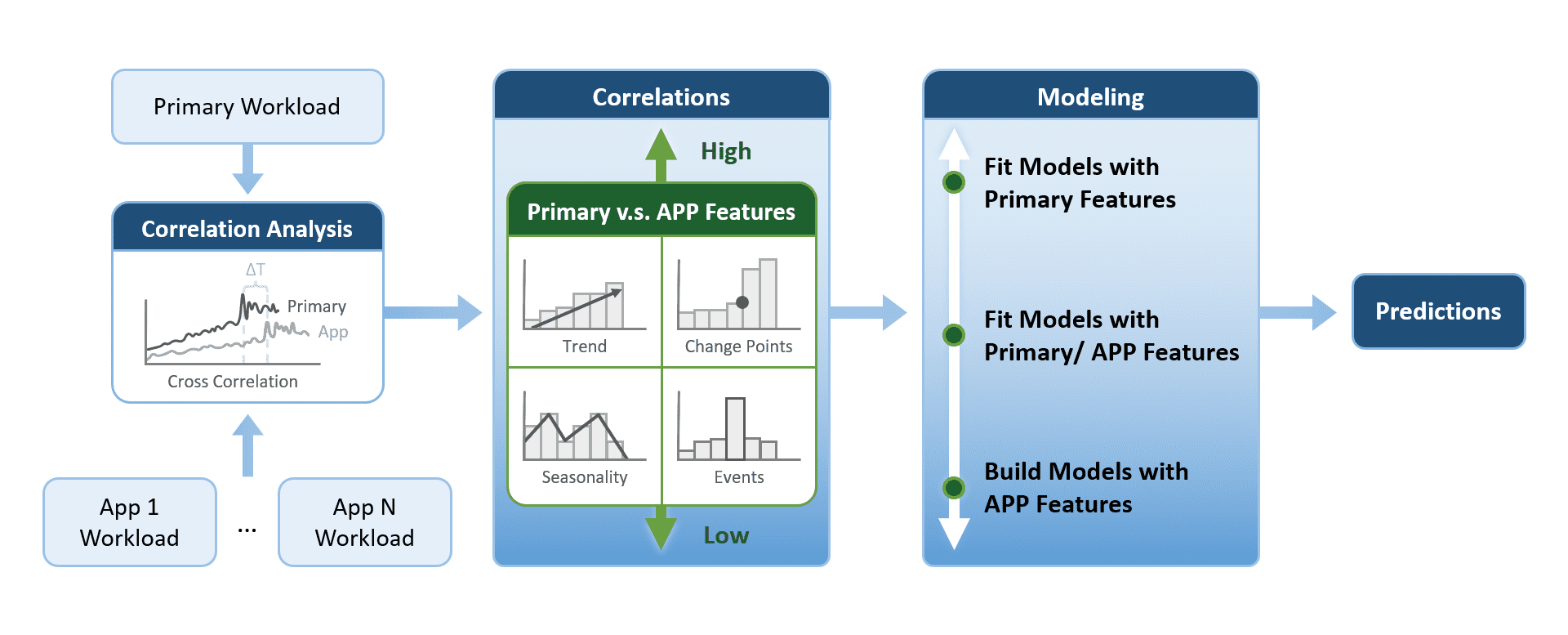
Figure 1 shows that communications among microservices form a communication graph, which illustrates the inter-dependency among these microservices. It is easy to see that the resource usage of these microservices will be impacted by the changing values of the primary workload, which is the web requests from the users. Here we propose a novel concept of prediction based on application correlations. More specifically, the prediction is based on the cross-correlation between the different workload patterns of microservices and the application’s primary workload. The proposed prediction algorithm has been implemented in ProphetStor’s CrystalClear Time Series Analysis Engine. Figure 3 illustrates the primary construct of the proposed prediction algorithm. With the input of the primary workload metric and resource usage metrics of microservices, the algorithm analyzes the dependencies between the primary workload and these microservice metrics by using cross-correlations. While a resource usage metric has a high correlation with the primary workload metric, it chooses a fitted model. It generates resource usage predictions based on the correlations and the features of the primary workload metric. Suppose a resource usage metric has a medium correlation or a low correlation with the primary workload metric. In that case, the system analyzes the application’s features (such as trend, seasonality, change points, events, etc.) and builds a suitable model for prediction generation.
Test Setups
1. Azure Function Traces in 2019 (called Azure2019 Dataset here).
- We use 3446-time series data from the traces – invocations per function for two weeks [7]. Each owner has several applications and functions which trigger different actions: HTTP, Timer, Event, Queue, Storage, Orchestration, and Others in Figures 5-a and 5-c.
- The primary workload time series is chosen by the time-series data with the maximum invocations, as shown in Figure 5-a.
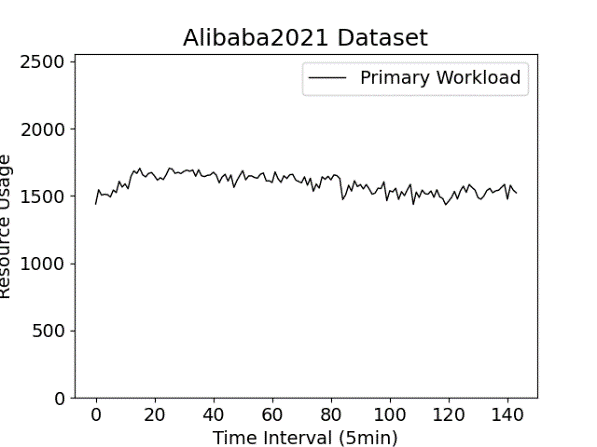
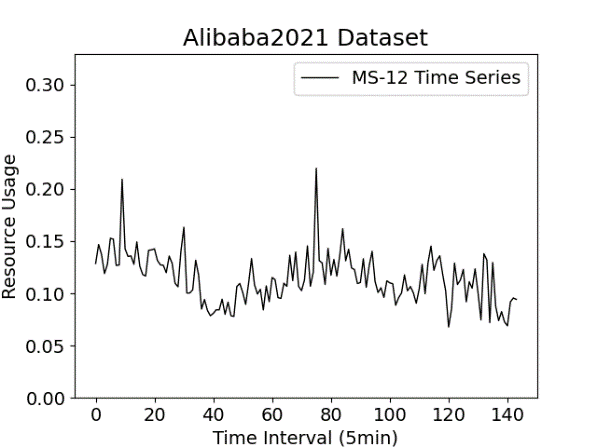
2. Microservices traces of Alibaba production clusters in 2021 (called Alibaba2021 Dataset here).
- We use 3899 time-series data, including CPU, Memory, and consumer metrics from 1303 microservices for 12 hours [8] in a production cluster in Figures 5-b and 5-d.
- We choose the time-series of CPU metric from a microservice with the highest CPU usage as the primary workload time series, as shown in Figure 5-b.
3. Figures 5-e and 5-f show the percentage of time series data with high cross-correlations between the primary workload time series and other time-series data in Azure2019 Dataset and Alibaba2021 Dataset, respectively.
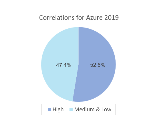
- For Azure2019 Dataset, as shown in Figure 5-e, only 53% of time series data with high cross-correlations (>=0.7), and 47% of time series data are medium or low correlations (<0.7). This is because these time-series data from serverless functions are of different owners.
- For Alibaba2021 Dataset, as shown in Figure 5-f, we can find that almost 95% of time series data have high cross-correlations (>=0.7) with the primary workload, and 5% of time series data have medium and low cross-correlations (<0.7) with the primary workload time series. The reason is that these microservices all work in the same production system and form a communication graph with a strong dependency.
4. Figures 5-g and 5-h show the two datasets’ characteristics of time series data.
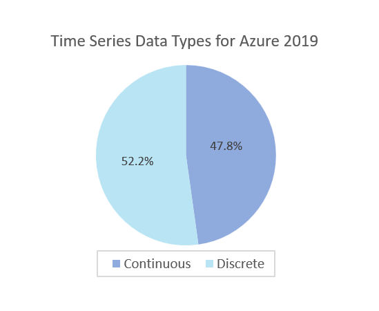
- For Azure2019 Dataset, as shown in Figure 5-g, about 52% of time-series data are discrete since users simply upload the code of their functions to the cloud, and functions are executed when triggered by events, such as receiving a message or a timer going off.
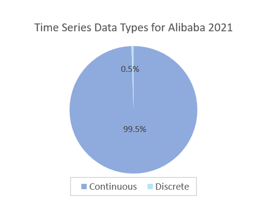
- For Alibaba2021 Dataset, as shown in Figure 5-h, only 0.5% of time series data are discrete, and most time-series data are continuous. Discrete-time series data bring multiple change points or unpredicted events. Therefore, they increase the difficulty of predictions and reduce the accuracy of predictions.


Exp 1. Perform predictions in the datasets with high cross-correlations (>=0.7)
Exp 2. Perform predictions in the datasets with medium and low cross-correlations (<0.7)
Exp 1: Datasets with High Cross-Correlation (>=0.7)
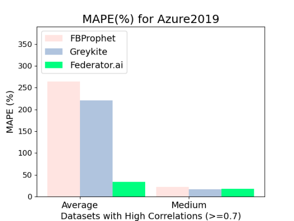

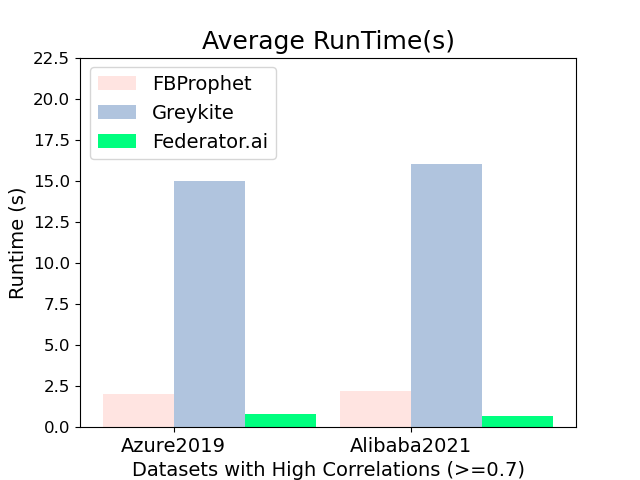
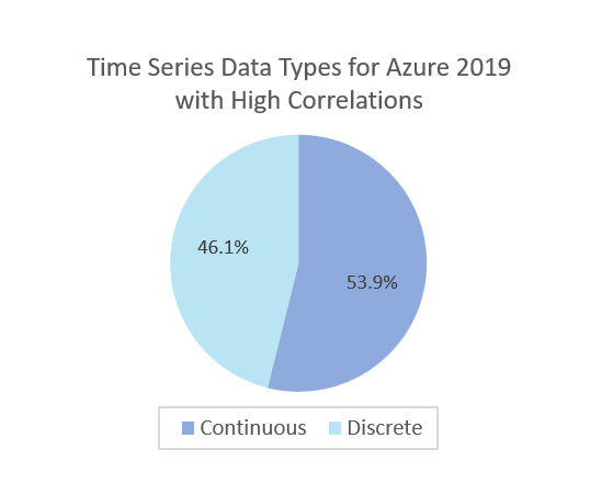
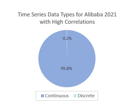
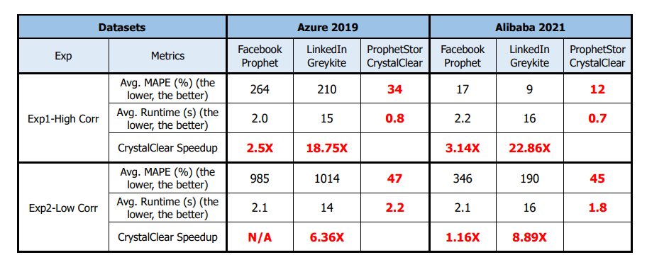
Figure Exp1-a shows the MAPE results of predictions for time series data with high cross-correlation in the Azure2019 dataset. In Figure Exp1-a, CrystalClear has the lowest average MAPE. The average MAPE values of FBProphet, Greykite, and CrystalClear are 264%, 221%, and 34%, respectively. The medium MAPE values of FBProphet, Greykite, and CrystalClear are 22%, 17%, and 18%, respectively. FBProphet and Greykite generate more outliers and obtain predictions with a higher average MAPE for time series data from the Azure2019 dataset. Almost 46 % of time series data are discrete, which increases more changepoints and unpredicted events for the Azure2019 dataset in Exp1-d.
Figure Exp1-b shows the MAPE results of predictions for time series data with high cross-correlation in the Alibaba2021 dataset. As shown in Figure Exp1-b, CrystalClear has a similar MAPE to FBProphet and Greykite. The average MAPE values of FBProphet, Greykite, and CrystalClear are 17%, 9%, and 12%, respectively. The medium MAPE values of FBProphet, Greykite, and CrystalClear are 10%, 3%, and 7%, respectively. All algorithms can achieve a lower average MAPE than that for Azure2019 Dataset. This is because most of the data in Alibaba2021 (99.8%), as shown in Figure Ex1-e, are continuous time series that would not generate changepoints and unpredict events to affect the prediction accuracy.
Figure Exp1-c shows the average runtime of a time series prediction by FBProphet, Greykite, and CrystalClear. CrystalClear achieves the lowest average runtime for both datasets since CrystalClear builds prediction models by considering cross-correlations of the primary workload time series and other time series. On the other hand, Greykite obtains the highest average runtime since it integrates more regressors and flexible functions to produce predictions. The average runtime of a time series prediction by FBProphet, Greykite, and CrystalClear for the Azure2019 dataset is 2.0s, 15s, and 0.8s, respectively. The average runtime of a time series prediction by FBProphet, Greykite, and CrystalClear in the Alibaba2021 dataset are 2.2s, 16s, and 0.7s, respectively.
Experiment 2: Datasets with Low Cross-Correlation (<0.7)

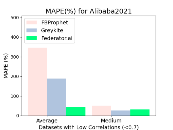
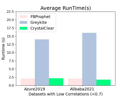
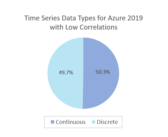
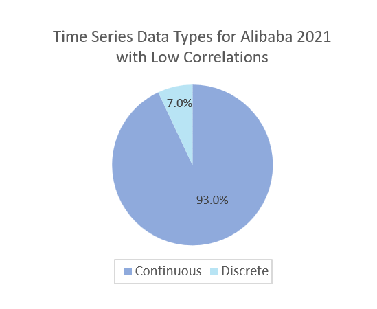
Figure Exp2-a shows the MAPE results of predictions for time series data with low cross-correlation from the Azure2019 dataset. In Figure Exp2-a, CrystalClear has the lowest MAPE. The average MAPE values of FBProphet, Greykite, and CrystalClear are 985%, 1014%, and 47%, respectively. The medium MAPE values of FBProphet, Greykite, and CrystalClear are 52%, 26%, and 32%, respectively. Figure Ex2-d shows that 50% of data (812 time series data) are discrete for the Azure2019 dataset. Because FBProphet and Greykite cannot handle discrete time series well, they generate many outliers and produce higher MAPE while making predictions for the Azure2019 dataset.
Figure Exp2-b is the MAPE results of predictions for time series data with low cross-correlation from the Alibaba2021 dataset. In Figure Exp2-b, CrystalClear has the lowest MAPE. The average MAPE values of FBProphet, Greykite, and CrystalClear are 346%, 190%, and 45%, respectively. The medium MAPE values of FBProphet, Greykite, and CrystalClear are 52%, 26%, and 32%, respectively. In Figure 2-e, we find that 7% of time series data in the Alibaba2021 dataset are discrete. Discrete-time series data generates multiple change points and unpredicted events.
Figure Exp2-c is the average runtime of a time series prediction by FBProphet, Greykite, and CrystalClear. We show that CrystalClear achieves similar average runtime for both datasets since CrystalClear builds prediction models by analyzing application patterns in these datasets with medium and lower correlations (<0.7). As shown in Figure Exp2-c, the average runtime of a time series prediction by FBProphet, Greykite, and CrystalClear for the Azure2019 dataset is 2.1s, 14s, and 2.2s, respectively. The average runtime of a time series prediction by FBProphet, Greykite, and CrystalClear for the Alibaba2021 dataset is 2.1s, 16s, and 1.8s, respectively.
Conclusions
Table 1 is the summary of the above results for different datasets. In summary, we know that the correlation-based prediction algorithm by ProphetStor’s CrystalClear archives a better prediction accuracy with smaller MAPE values and a lower average runtime than that of FBProphet and Greykite when there are high cross-correlations among the primary workload metric and other metrics. With CrystalClear, the cost of workload prediction tasks is reduced up to 3.14X compared to the runtime of FBProphet, and up to 22.86X compared to that of Greykite.
We believe most microservice-based applications would exhibit the same high level of correlation among metrics from microservices within an application. With a correlation-based prediction algorithm, CrystalClear quickly generates a large number of forecasts with high accuracy and provides a low-cost solution for resource management for microservices.
References
[1]. Shutian Luo, et al. “Characterizing Microservice Dependency and Performance: Alibaba Trace Analysis. In ACM Symposium on Cloud Computing (SoCC’ 21).” November 1–4, 2021, Seattle, WA, USA. ACM, New York, NY, USA, 15 pages.
[2]. Mohammad Shahrad, et al. “Serverless in the Wild: Characterizing and Optimizing the Serverless Workload at a Large Cloud Provider.” in Proceedings of the 2020 USENIX Annual Technical Conference (USENIX ATC 20). USENIX Association, Boston, MA, July 2020.
[3]. Box, G.E.P. and Jenkins, G. 1976. “Time Series Analysis, Forecasting, and Control.” San Francisco: Holden-Day.
[4]. “Forecasting at scale.” https://facebook.github.io/prophet/
[5]. “Greykite: A flexible, intuitive and fast forecasting library.” https://github.com/linkedin/greykite
[6]. Hosseini, Reza, et al. “A flexible forecasting model for production systems.” arXiv preprint arXiv:2105.01098 (2021).
[7]. “Azure Functions Trace 2019.” https://github.com/Azure/AzurePublicDataset/blob/master/AzureFunctionsDataset2019.md
[8]. “Overview of Microservices Traces.” https://github.com/alibaba/clusterdata/blob/master/cluster-trace-microservices-v2021/